A few weeks ago, I helped optimize some training runs at work. Each model was quite small, no more than 50M parameters, yet took 12+ hours to train on an A100 GPU! While debugging, I learned about JIT compilation, rooflines, and how best to squeeze performance out of hardware that’s designed for models 100x the size. I wrote up some thoughts on the topic and hopefully they’ll be useful to you as well.
Idiosyncrasies
There are a number of resources focused on optimizing training runs for models with billions of parameters sharded across multiple devices. The same high-level principles follow for small models, namely designing model architectures that match the hardware they run on; however, small models experience a few unique problems:
Thanks for reading ross's archive! Subscribe for free to receive new posts and support my work.
Forward and backward passes are short, which make them sensitive to framework overhead (eg. kernel launches).
Levers for increasing a model’s FLOPs, namely batch size, can degrade its quality, particularly when training data is scarce.
With that in mind, the following sections will cover strategies for measuring performance and optimization techniques, coupled with experiments demonstrating their effectiveness.
Measurement
Note.FLOPs and FLOPS will be used extensively. The former denotes floating-point operations, while FLOPS describes a rate: floating-point operations per second.
With small training runs, we often care the most about speed; other operational metrics, such as availability, are less critical because runs are short and typically rely on a single GPU / TPU.
Metrics are ordered by increasing granularity. More granular metrics provide insights into how the hardware is being used but are also hardware-dependent and often volatile.
Projected Run Duration (PRD)
Projected Run Duration is the projected duration of a training run at a point in time, and is commonly computed from an averaged steps-per-second rate:
PRD is the starting point for optimization and is readily computed by loop trackers like tqdm. Assuming the run duration is acceptable, it may be more productive to work on something else in the meantime, at the expense of wasted compute cycles!
As a rough heuristic, PRD should roughly match a proportion α of the minimal duration given your compute hardware:
\(\frac{\text{Remaining Model FLOPs}}{\text{Accelerator FLOPS}} = \alpha \cdot \text{PRD}\)
If alpha is large, it may be worth investigating further. More on this in the next section!
Model FLOPs Utilization (MFU)
Model FLOPs Utilization measures the amount of FLOPs used for forward and backward passes over a time window t divided by the hardware’s FLOPS rate:
You may have noticed that the heuristic mentioned in the previous section is essentially MFU. This metric was introduced by Google’s PaLM paper and attempts to provide a hardware-agnostic measurement of useful FLOPs for a training run, ignoring any FLOPs used for memory optimizations such as gradient checkpointing.
Model FLOPs is often approximated by viewing a model as a collection of linear layers of the form:
In this approximation, each layer requires 2BDF FLOPs for the forward pass via a single matrix multiplication and 4BDF FLOPs for the backward pass, totaling 6BDF FLOPs.1 Aggregating over all layers, we obtain:
This approximation is fairly tight for short-context transformers and MLPs, and thus sufficient for our use case!
Hardware FLOPs Utilization (HFU)
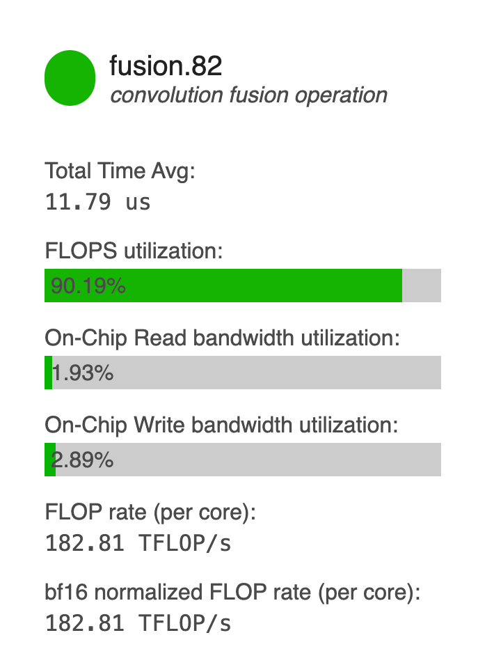
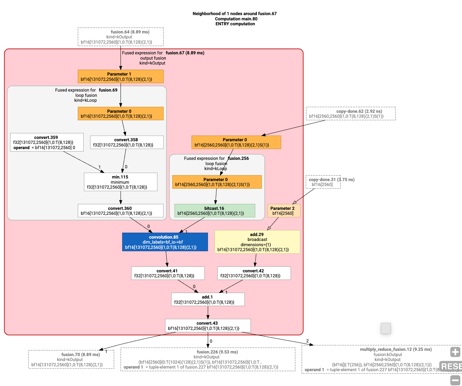
Fusion-level HFU utilization measured by the JAX profiler.
Hardware FLOPs Utilization measures the proportion of hardware FLOPs utilized at a point in time or over an interval. HFU may be measured at a range of scales: an entire training run, several steps, or a single operation invocation (eg. kernel or fusion). Step-level HFU is computed using FLOPs estimates, similar to MFU.
Observing operation-level HFU requires configuring a profiler but is invaluable for optimizing training loops, as high HFU is necessary but not sufficient for high MFU. In general, I’d recommend profiling a baseline training loop, identifying bottlenecks, and optimizing from there! 2
Optimizations
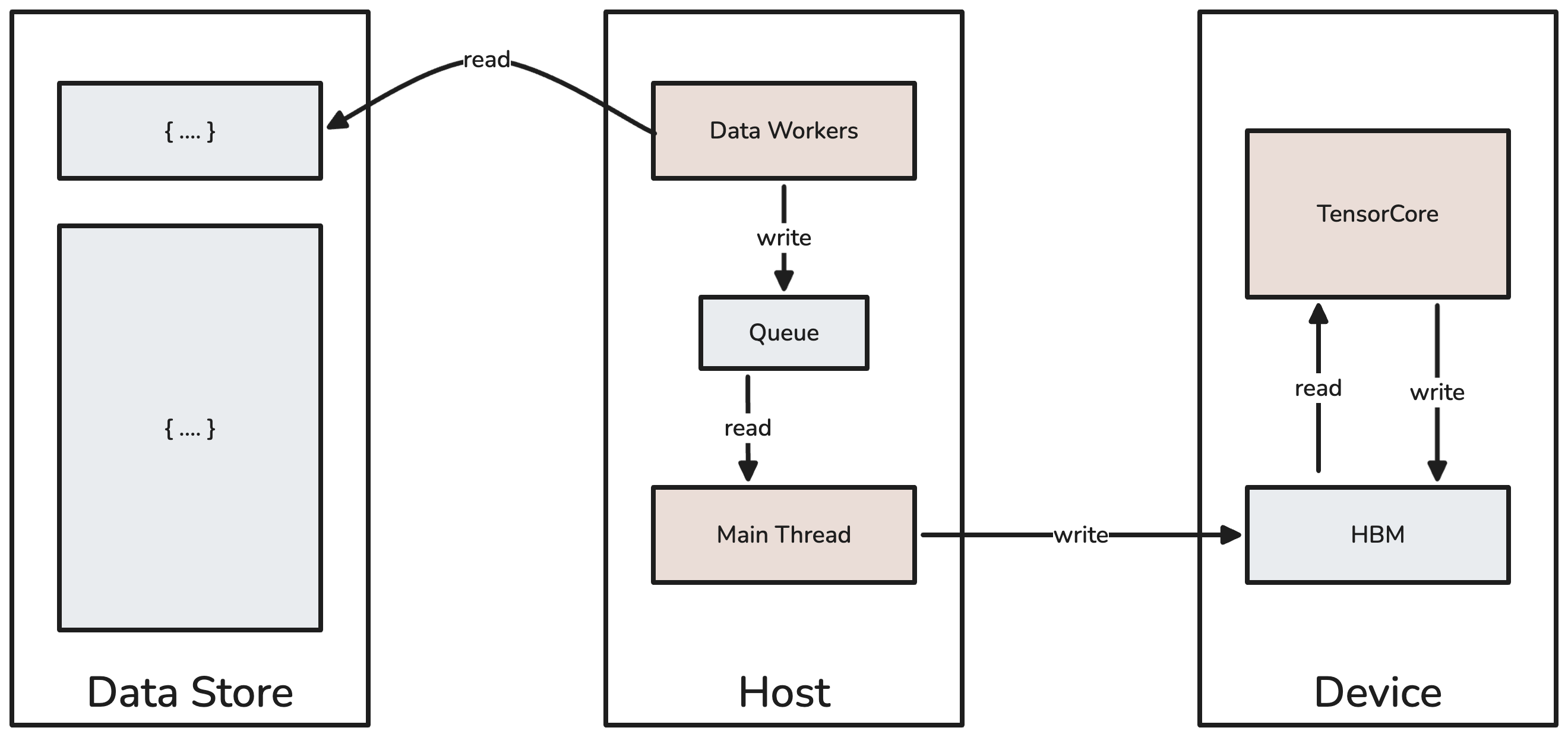
A high-level view of the typical training pipeline, which moves data from data stores (eg. NVMe SSDs, AWS S3) to a host and from host to device. High-bandwidth memory (ie, HBM) is the device’s main memory block.
Ensuring Compute-Boundedness
TPUs and GPUs can execute hundreds-to-thousands of teraFLOPs per second; however, compute throughput is only utilized if there are bytes available to process. And so the performance of a training pipeline is contingent on:
The ability to overlap data transfers with compute, ie. data transfers happen independently of compute.
Computation duration exceeding data transfer duration, ie. communication, for all components of the pipeline.
Without overlap, computation is serialized on data transfers and cores are left idle, and the same is true if communication takes longer than computation.
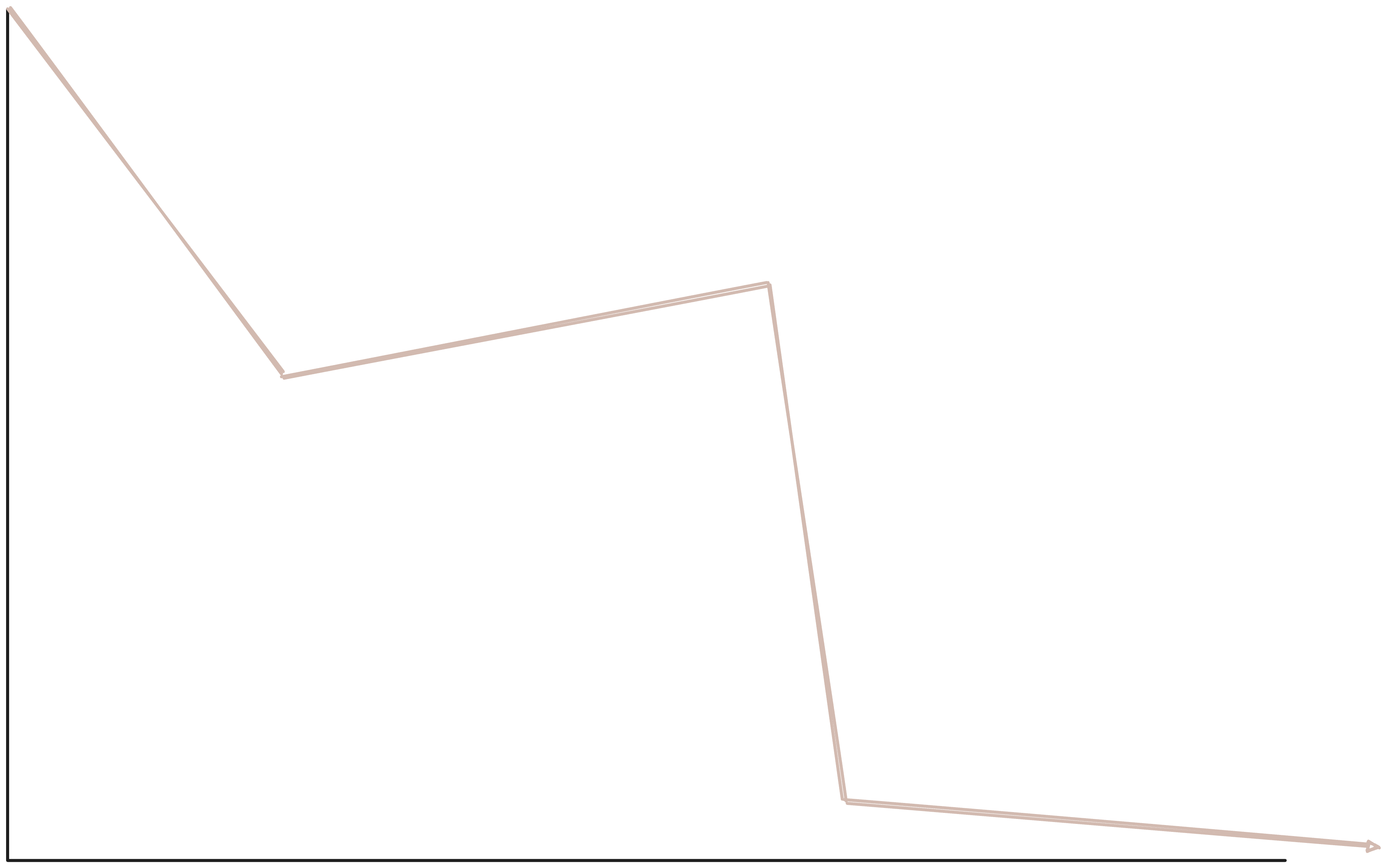
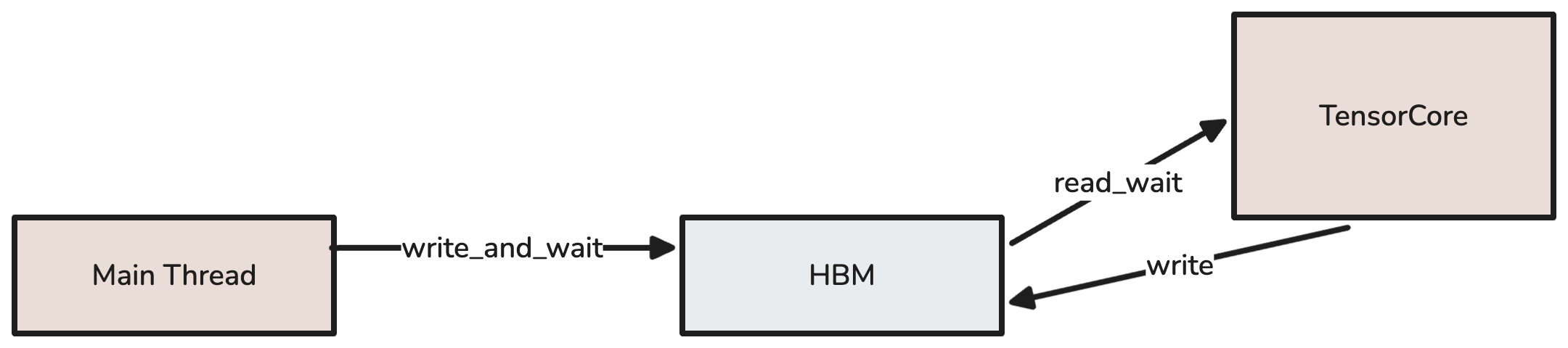
A simplified example of non-overlapped communication. The Main Thread waits on device results, and symmetrically the TensorCore waits on fresh data.
In practice, overlap is achieved by asynchronous data transfers between components:
Data Store → Host: worker processes on the host prefetch batches and add them to an in-memory queue.
Host → Device: the main thread reads a new batch and writes it to the device’s HBM over PCIe.
HBM → TensorCore: the TensorCore loads data from HBM and applies matrix and vector operations. 3 Load instructions are pipelined and interleaved with compute.
Assuming compute and data transfers are overlapped, compute boundedness reduces to comparing compute and communication durations:
The right-hand side is dependent on the accelerator and data transfer type, but is otherwise fixed. As an example:
HBM → TensorCore transfers use very fast interconnect, on order of 8.1e11 bytes/s for v5e TPUs; Host → Device relies on comparatively slower PCIe at 1.6e10 bytes/s.
Assuming our model uses bfloat16 for forward and backward passes, v5e TPUs provides 1.97e14 FLOPS. For HBM → TensorCore, the left-hand side becomes 1.97e14 / 8.1e11 ~= 243; similarly, Host → Device yields 1.97e14 / 1.6e10 ~= 12312.
In general, if a data transfer yields more FLOPS per byte than the hardware’s Accelerator FLOPs / Comm. Bandwidth ratio, then it’s compute-bound, otherwise it’s communication-bound; intuitively, this ratio is the data “fill rate” at which the accelerator always has new data to process.
Small models are often pushed into communication-bound regimes due to small batch sizes, insufficient model width or depth, or low bandwidth for Data Store → Host transfers. And so it’s important to understand whether your hardware or architecture are limiting performance.
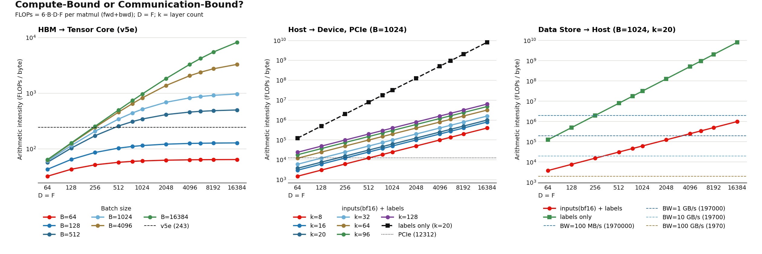
A roofline analysisof how batch size (B), MLP layer count (k), and hidden-layer size (F) determine whether our model is compute or communication bound. For simplicity, we assume that D = F. Horizontal dashed lines represent communication-to-compute transition points.
Roofline plots are used for identifying communication bottlenecks in training pipelines, and visualize the relationship between a free parameter (eg. batch size or model width) and its impacts on compute-intensity, measured in FLOPs per bytes. Let’s look at a concrete example!
The plots above provide rooflines for a multi-layer (k) MLP with batch size (B), hidden dimension (F), and a input dimension (D); bfloat16 is used for weights, activations, and gradients. The MLP requires 6BDF * k FLOPs per step, and transfers a variable amount of bytes depending on the data transfer:
HBM → TensorCore data transfers move model weights and activations to-and-from HBM three times per step, or 3 * 2 * (BD + DF) bytes per layer. Therefore, the ratio of FLOPs to bytes of is 6BDF * k / 6k * (BD + DF) = BDF / (BD + DF). When B is small, this expression is roughly B, and is symmetrically F when F is small.
Using this formula, we can construct a roofline plot! The left roofline plot highlights how compute intensity varies with batch size and model width, and the horizontal line marks the transition between communication-bound v. compute-bound regimes for a v5e TPU. Since HBM is high-bandwidth, even very small models (eg. F=D=512) may be compute bound provided a sufficiently large batch size.
Host → Device data transfers move inputs and targets over PCIe, or 2BD + 4B bytes per step — assuming bfloat16 inputs. Therefore, the ratio of FLOPs to bytes is 6BDF * k / 2BD + 4B ~= 3kF. In the case of auto-regression LLMs, inputs and labels are identical and so only 4B bytes are moved, yielding a ratio of 6BDFk / 4B = (3/2)DFk. Notice how increasing a model’s batch size does not impact FLOPs per byte.
The middle plot highlights how model width and depth impact compute intensity for PCIe transfers. Small models must be sufficiently wide or deep to achieve compute-boundedness, particularly when input embeddings are transferred. A 20-layer MLP, for instance, requires F > 256 to be compute-bound.
Data Store → Host data transfers move inputs and targets over TCP or PCIe. Transfer bandwidth varies widely between the hardware used. For instance, PCIe-based NVMe SSDs support multi-GB/s reads while AWS S3 support ~100 MB/s per connection, relying on multiple connections to achieve high throughput. Both Host → Device and Data Store → Host share the same payload size and consequently have the same FLOPs per byte value.
The right plot highlights how transfer bandwidth impacts rooflines for a model with varying width but fixed depth. If inputs and labels are identical, a model is compute-bound with a relatively modest hidden dimension of > 256 and 100MB/s bandwidth. Conversely, models with embedding-valued inputs are compute-bound at the same hidden dimension only if Store → Host bandwidth is 10+ GB/s. Even the fastest NVMe SSDs may struggle to keep up in this scenario!
The takeaway is that small models are often at a risk of being communication-bound, though there are several levers we can pull:
Increasing batch size improves FLOPs utilization for HBM → TensorCore transfers, but has a negligible impact on other transfer types.
Communication-bound PCIe and data store transfers require increasing either model depth or width. A sufficiently small model cannot overcome low-bandwidth links; this is more of a concern for data store transfers, and may be mitigated by prefetching batches across multiple workers or upgrading local disks. 4
Realizing Overlap
As mentioned in the previous section, achieving high FLOPs utilization requires overlapping compute and communication. Fortunately, PyTorch and JAX support this execution model out of the box via asynchronous execution, also known as asynchronous dispatch.
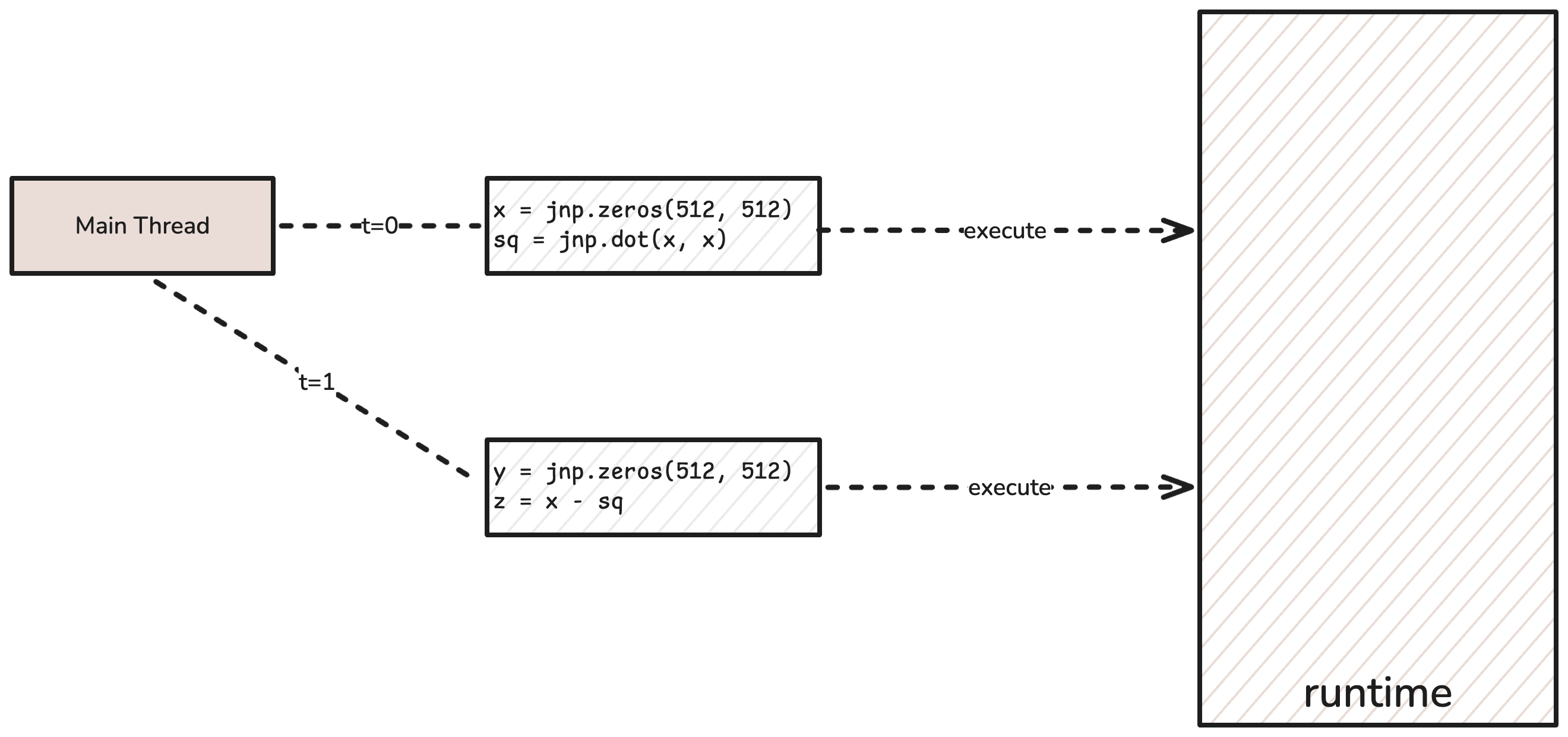
Async dispatch for a four-line JAX program.
If you’re familiar with asynchronous programming, the semantics are nearly identical. Each tensor operation is sent to the framework runtime and is executed in the background. From the caller’s perspective, operations return immediately and the response tensors acts as a future, which may in turn be composed with other operations.
This behavior is very useful for overlapping data loading with training steps. Consider the following example:
...
for step in range(steps):
  # move to device
  batch = jax.device_put(get_batch(step))
  loss = train_step(model, batch)

# print the final loss
print("final loss: ", loss)
...
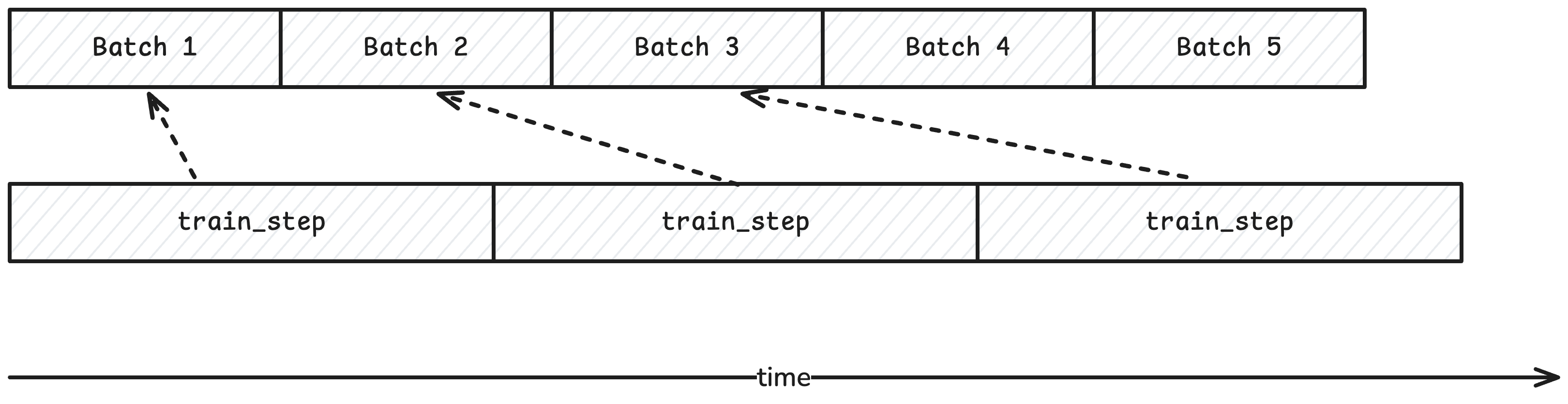
Here train_step executes asynchronously and the loop proceeds to the next step. The loop only blocks if it depends on a device tensor result, which is the print statement in this example. Here we achieve perfect overlap because all batches are loaded on the device while train_step invocations execute:
A view into how the device’s execution lags batch loads into HBM.
Introducing monitoring or checkpointing, however, can discount these benefits. Consider logging the loss per step:
...
for step in range(steps):
  # move to device
  batch = jax.device_put(get_batch(step))
  loss = train_step(model, batch)
  # print the step loss
  print(”step loss: “, loss)
...
Now, each step must wait on the result of train_step, serializing data transfers and training steps. The most common solution is to defer logging for losses, gradient norms, and other device tensors for several steps — the intuition being that tensors will be ready for device-to-host transfers after some duration:
...
last_loss = None
for step in range(steps):
  # move to device
  batch = jax.device_put(get_batch(step))
  loss = train_step(model, batch)

  # defer logging for one step
  if last_loss:
    print(”previous loss: “, last_loss)
  last_loss = loss
...
As an aside, overlap may also suffer if the training loop has to handle CPU-intensive operations, such as model checkpointing, though this is less of a concern for small models.
JIT Compilation
Another very important tool is JIT compilation, which compiles a sequence of tensor operations into optimized, fused kernels. For instance, an expression like relu(x* W + b) may be fused into a single kernel instead of three:
A fused kernel for relu(x* W + b)compiled from JAX via XLA.
JIT compilation is particularly advantageous for small models because it reduces framework overhead. Each kernel launch requires tensor allocations, copying executables to HBM, tensor copies, and other operations —totaling tens-to-hundreds of microseconds per step. For a 20M MLP on a v5e TPU, overhead can easily exceed compute time!
One clever use of JIT is to compile multiple training steps into a single executable:
def training_step(model, batch, step):
    loss, grads = jax.value_and_grad(
      lambda m: m.loss(model_hparams, train_hparams, batch)
    )(model)
    ...
    return model, loss

# a jit-compiled version of `steps` steps
@jax.jit
def train_with_steps(model, batches, steps):
  # batches is a list of batches
  def scan_step(model, scan_inputs):
    batch, step = scan_inputs
    return training_step(
      model, batch, step, model_hparams, train_hparams
    )
  # apply training_step per batch
  return jax.lax.scan(scan_step, model, (batches, steps))
With this approach, JAX compresses the overhead of several executable launches into a single launch, at the cost of increased HBM usage. For small, latency-bound models, this technique recovers MFU that would otherwise require raising the batch size.
Experiments
This section explores how the optimizations discussed above impact MFU for a family of MLPs with ReLU activations. A few notes on the experimentation setup:
Each MLP has a hidden dimension of 1024, and the input dimension is also fixed at 1024. Model depth is adjusted to achieve desired parameter counts per experiments.
All models were trained on a synthetic classification task. Data is generated by randomly sampling vectors from a normal distribution, and classes are determined from a vector’s norm. Batches were sampled on-device as opposed to using host-to-device transfers.
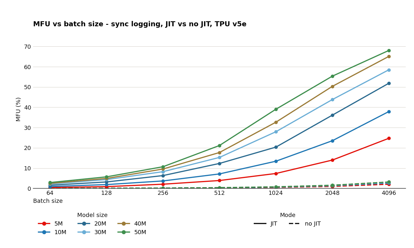
JIT compilation yields a significant performance bump across all models. Uncompiled models realize <1% of MFU.
What is the impact of JIT compiling models? For small models, fusing a model’s hundreds of operations leads to a significant improvement in MFU. Even with large batch sizes, uncompiled models struggled to exceed 5% MFU, and a 20M parameter compiled model should expect to see a ~10% lift in MFU at moderate batch sizes.
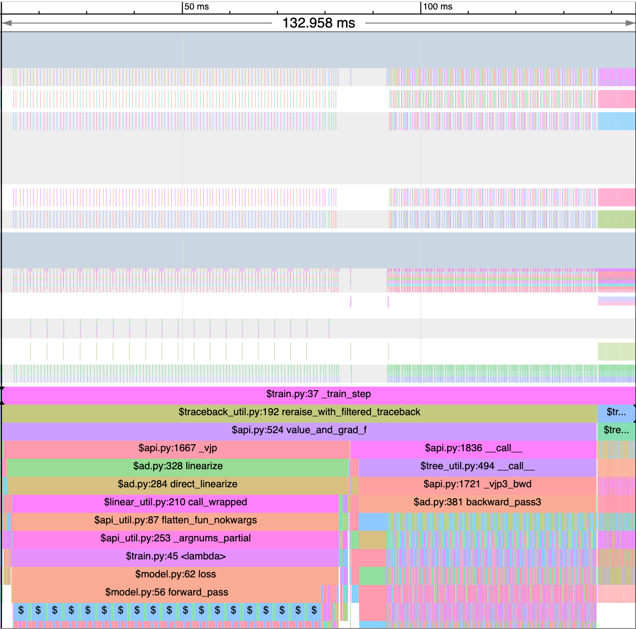
What causes a divergence in MFU between JIT and no-JIT models?
No-JIT models (top) are very slow. A training step for a ~20M-parameter MLP takes over ~130ms but may be fused (bottom) into a single, sub-millisecond train step.
The primary reason is overhead. An uncompiled model has to dispatch each add or matmul operation independently, and moving data to and from HBM hundreds of times incurs significant overhead. You can see this in the trace above, where JIT smooths many discrete operations into a nearlyuniform executable.
The main takeaway from this experiment is that JIT compilation often provides easy performance wins with minimal effort and is worth experimenting with early on!
Experiment 2: Multi-Step JIT
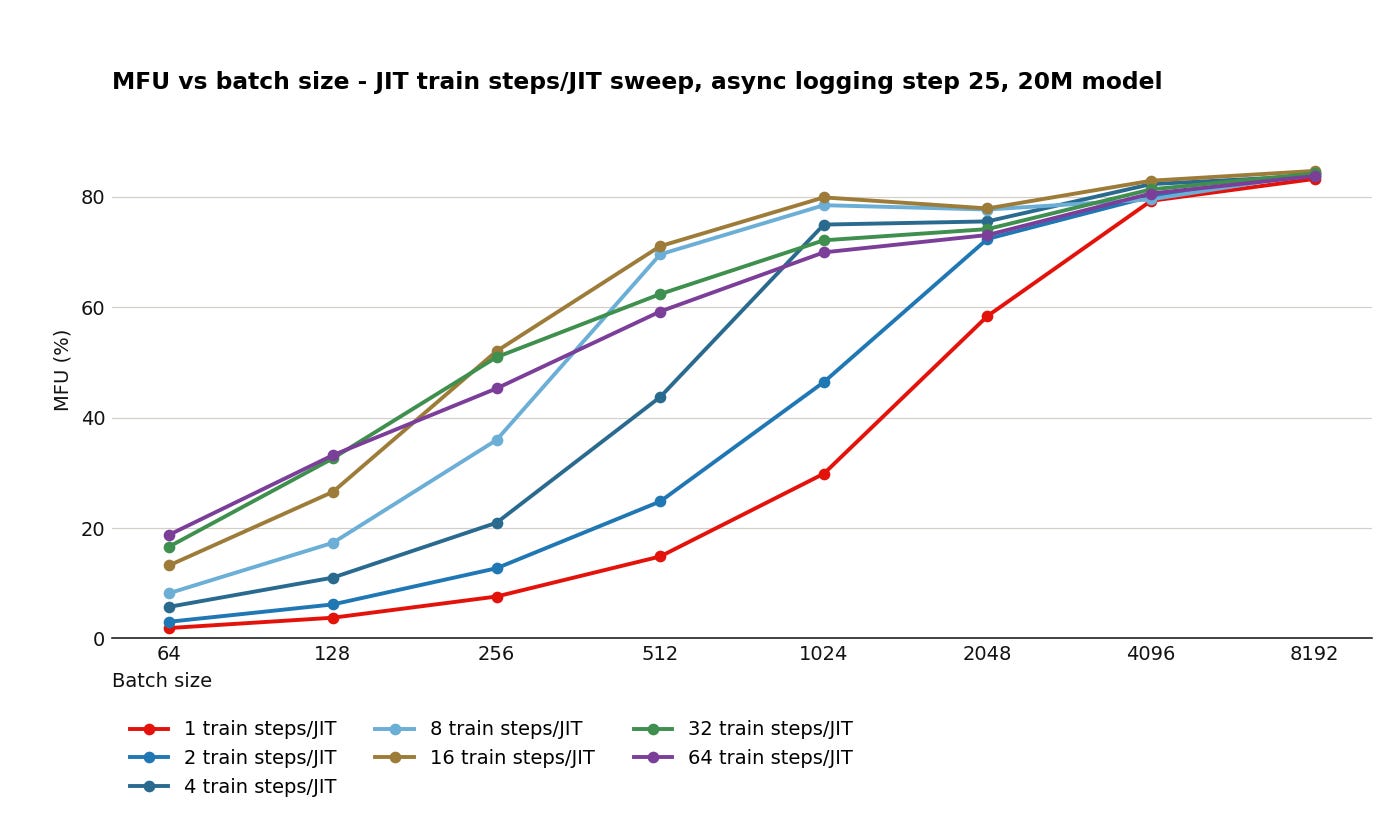
Fusing train steps tends to help MFU performance; note that variance between runs is high.
Does JIT compiling multiple training steps improve MFU for small models? In our testing, yes! For a 20M parameter MLP, fusing multiple train steps leads to 15-20% lift in MFU, though gains taper off at around 16 steps per JIT.
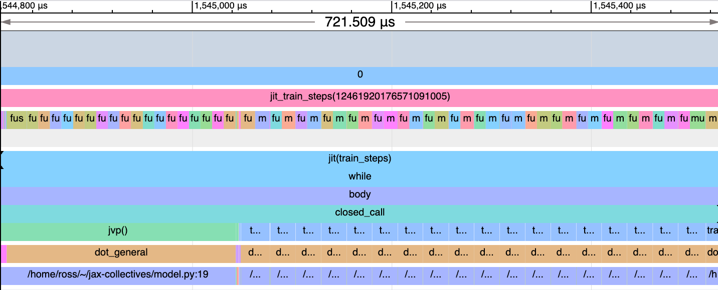
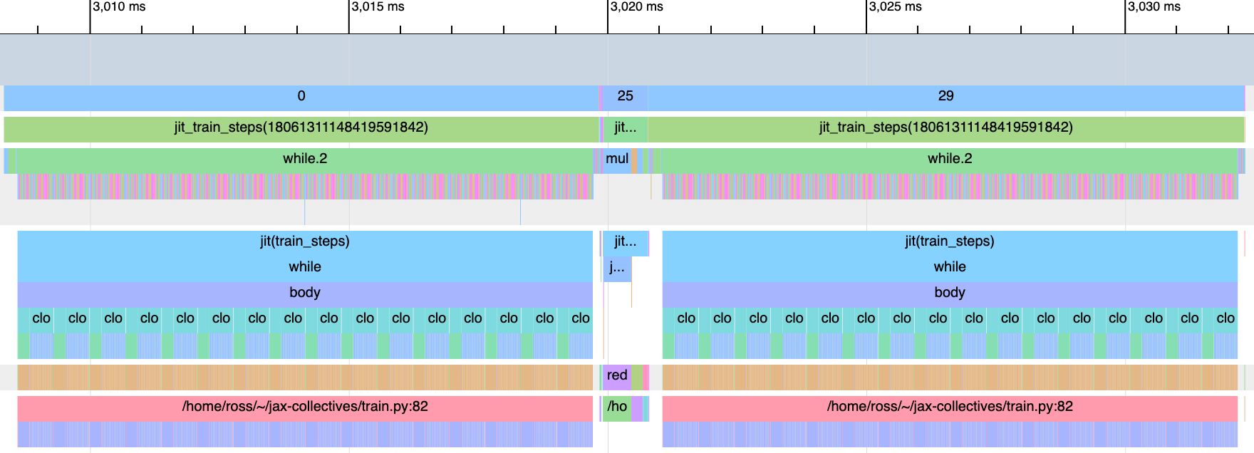
Fusion is implemented by scanning over train steps for a fixed step size, which yields longer kernels compared to baseline:
Fusion is implemented as a jax.lax.scan over train steps. This trace is from a 20M parameter MLP.
This optimization, however, is constrained by communication bandwidth. Namely, the amount of training data transferred over PCIe scales linearly with the JIT step size, meaning communication-bound training loops will not benefit.
Conclusions
Small models struggle to saturate compute on modern hardware, often due to communication-bound training loops or host overhead. However, substantial progress can be made by understanding a few core ideas: compute and communication must overlap, compute duration must be the long pole, and rooflines are your map!
The backward pass requires computing dL/dW and dL/dIn, each of which follow the same shaped matrix multiplication as the forward pass: np.dot(dL/dOut, W) and np.dot(dL/dOut, In). See this reference for a derivation.
For object stores, prefetching can improve throughput by opening multiple connections per worker, up to the network bandwidth of your host. Each connection supports ~5Gbps, or 625 MB/s, though this number is almost always lower in practice. Host-level bandwidth limits depend on the instance type but ranges from 25-100 Gbps.

This is awesome!!